
As published in Converting Quarterly in Quarter 3, 2021 by E.J. (Ted) Lightfoot, Ph.D., principal, Ted Lightfoot LLC.
The best-known process map in the converting industry is the coating window. There are three stages to managing the coating window. First, map the boundaries (constraints) of the process. Second, determine where within these constraints the process runs best. Finally, the coating engineer becomes responsible for managing the formulation and process to optimize the fit of the process to the needs of the business.
Introduction
The first thing to teach a new coating engineer is how to be safe. The second thing to teach a new coating engineer is how to manage the coating window. Most people in the industry understand coating windows as maps of operating parameters that produce nominally uniform coating. The boundaries of the coating window delineate the regions of parameter space beyond which gross defects of one sort or another occur. Because this is one of the first things people learn, the explanation often is simplified to “as long as you are inside the coating window, things are good; if you are outside the window, things are bad.” This oversimplification can be extremely costly.
There are three reasons being inside the window is not enough. First, you usually want to maximize productivity rather than take the first line speed that worked. Second, while coating windows are drawn as two-dimensional maps, many parameters affect the shape of the window. Understanding and monitoring the boundaries of the coating window allow you to expand the coating window (which comes back to productivity). Finally, variations in the uniformity of the coating made in different parts of the coating window usually create a “sweet spot” within the window.
Coating windows may be specific (with numerical scales) or generic (topological renderings showing the defects bounding each part of the window). For example, Coyle [1] gives experimental windows for the metering gap of a reverse-roll coater showing the onset of ribbing and cascade defects but generic windows that show the onset of starvation, vortex instabilities, run-back and air entrainment in the pan. It is important to document the specific window for a new product for future troubleshooting [2].
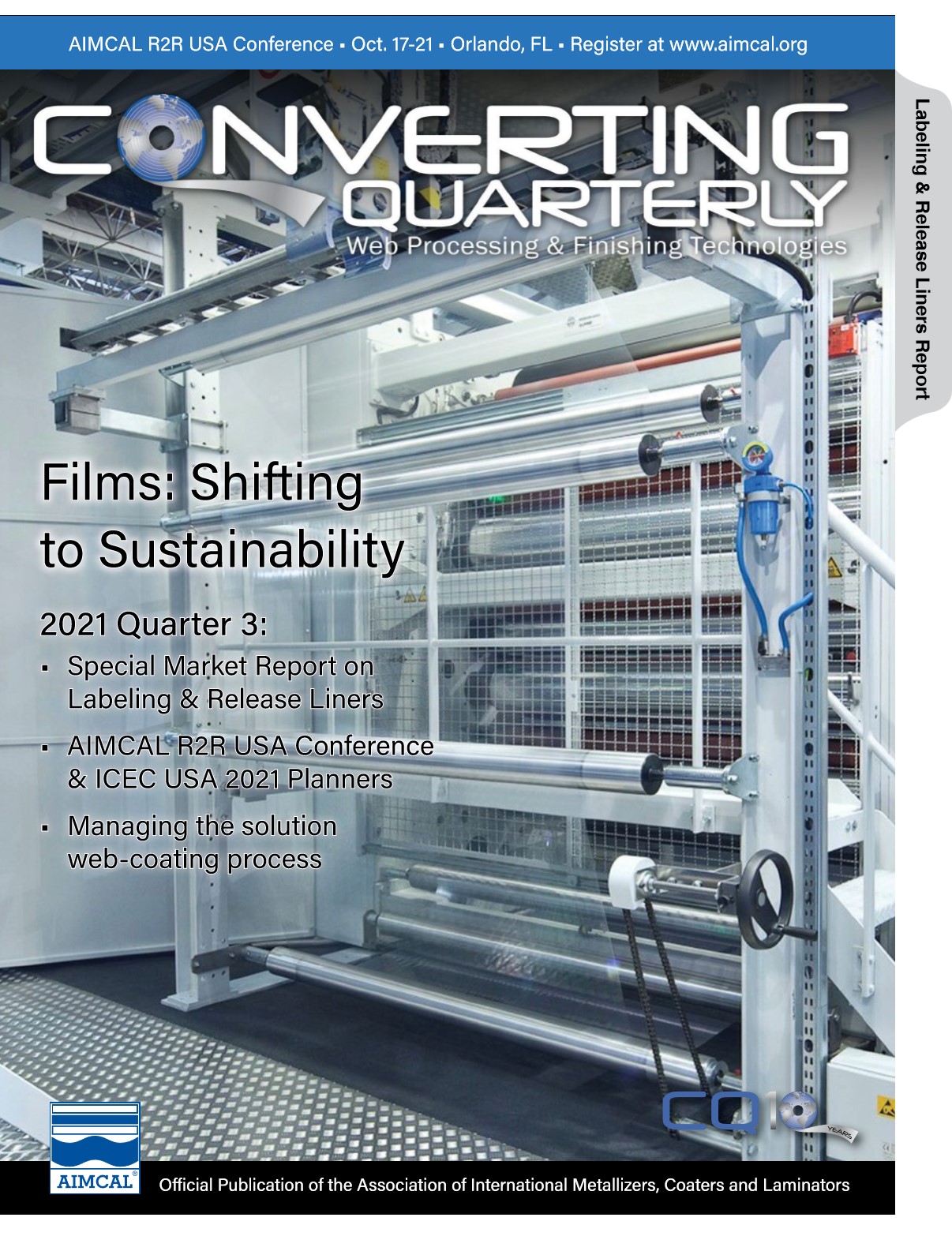
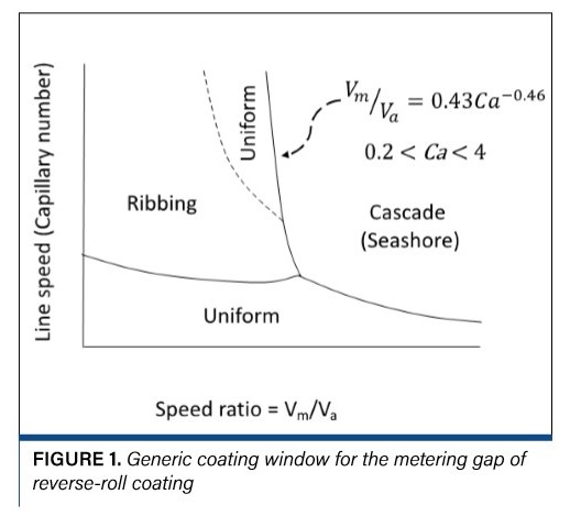
Specific windows for existing products become generic windows to help you plan new product development. Figure 1 gives a generic window for the metering gap of a reverse-roll coater with a correlation for the transition from uniform flow in cascade given by Coyle [1]. The onset of ribbing is gradual, but the onset of cascade is fairly sharp, so most people run closer to cascade than ribbing. But the speed ratio Vm/Va (along with the gap) is used to control the coating thickness. So, you want to set the gap, constrained by the cascade limit, to run in a range of metering-roll speeds that produces good quality and control. Understanding the dependence of the cascade constraint on formulation helps you maximize line speed.
How to map the perimeter of the coating window
The most robust maps are experimental. Mapping is done in two phases: map the perimeter, then map the center. This is analogous to producing a contour map of an island. You need to know where the land ends and the water begins; you want to know how high the land is, and you want to understand the effects of tides (hysteresis). It is easiest to visualize a two-dimensional map, so it is customary to map two or three parameters at a time. The most common maps use line speed as one of the independent variables. Depending on the coating method, typical additional variables are roll-speed ratios, vacuum level, angles, viscosity, pressures, coating-head geometry and gap.
Mapping the perimeter requires a different approach than mapping the center. To find the boundaries, process settings are varied one at a time until a gross defect occurs. Efficiency is important: Scan in a way that you expect to give the fastest cycle time. The high-speed gap in Figure 1 is relatively narrow. It is more efficient to set the applicator roll and line speeds while varying the ratio than to set the ratio and vary the line speed (you also want to measure the coatweight response at constant applicator and line speed). For a coater with a vacuum box, it is faster to scan the range of vacuum than vary the line speed. Lay out a reasonable range of line speeds, at each speed find the width of the window and repeat. If you want to measure the effect of other variables, you can repeat this sequence at various levels of the additional variables.
Slot-die coating with a vacuum box
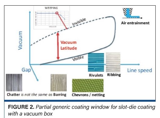
The fastest-growing coating method is slot-die coating with a vacuum box. Figure 2 shows a partial generic coating window for this system. There are other defect patterns not shown as well as vortex instabilities that cannot be illustrated in this view. Ding, et al [3], review the common defects and known limits for this system.
Of particular interest are the Higgins Scriven visco-capillary approximations of the upper and lower vacuum limits of the process. These apply only in the limit of low inertia and require an estimate of the dynamic contact angle (not a widely available measurement).
However, you can treat the dynamic contact angle as an adjustable parameter to correlate data. Viscocapillary theory predicts the vacuum latitude to be twice the surface tension of the upstream meniscus divided by the upstream die-to-web gap (if the meniscus is pinned at the upstream corner of the die). Are these estimates reliable? No. Are they useful? Extremely. The visco-capillary model is asymptotically accurate for low inertia but not at higher speed.
However, the bigger issue (for any theory) is the condition of the die. When the die is in perfect condition with edges sharpened to a radius of no more than a few microns, the upstream meniscus is likely to be pinned at the upstream die edge. If the sharp radius becomes worn, the meniscus is likely to move and wet the upstream (and/or the downstream) face of the die. If this happens, the coating window will change. This is why it is important to check the coating window periodically. Unfortunately, the weeping that occurs above the upper vacuum limit can be hard to see (often the coating is nominally uniform, but the coatweight is low). The most robust way to measure the upper vacuum limit is to coat patches at different vacuums, check the quality and measure the coatweight at each vacuum to see when the coatweight starts to drop. A simpler approach is to measure the lower vacuum limit every time you cast off and control-chart the result.
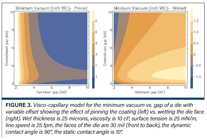
Another way to check for changes is to measure the minimum vacuum vs. gap. Figure 3 compares viscocapillary predictions of the minimum vacuum limit for coatings that are pinned or wet the face of an off set lip die. For a pinned coating, the lower vacuum limit drops as the gap increases; for a coating that wets the die, the lower vacuum limit increases as the gap increases. No matter your speed range and how you measure changes, tracking changes to the boundaries of the coating window can tell you when the die needs to be reworked.
One complication with mapping the boundaries is hysteresis. Some defects come and go at well-defined points, other defects come and go at different points depending on whether the parameter is increasing or decreasing, hence coaters can operate in regimes where the defect may or may not occur. For example, the coating may be smooth or have one or more defects, depending on if it wets the die face, is pinned at the edge of the die or pinned at the edge of the slot. You may be able to establish a uniform coating by shimming the gap to move the pinning point, but eliminating the defect with vacuum may require a large change to move the meniscus. From a mapping standpoint, record the transition both increasing and decreasing and plot both (think of this as recording the island’s shoreline at low and high tides). If you want to control-chart the variable (e.g., minimum vacuum), you want to record the greatest extent of the window (e.g., look at the point in which the uniform coating breaks down as the vacuum is decreased).
Mapping the response surface
The second stage in mapping is assessing the attractiveness of the points inside the window. In some cases, the coating just needs to be present; the only goal is productivity. In other cases (e.g., reverse-roll coating), the coatweight varies across the window, and you want to maximize productivity subject to the constraint of having the right coatweight. In still other cases, coatweight variations are problematic, and you want to “co-optimize” productivity and uniformity subject to the constraint of getting the right coatweight.
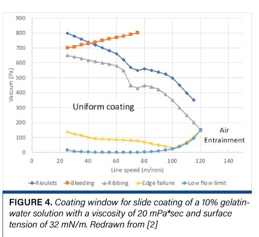
The most detailed specific window in the open literature is the slide coating window given by Hens [4] (redrawn in Figure 4). The lines and the point of air entrainment represent the onset of six gross defects in the coating while the central region is labeled “uniform coating.” But because slide coating was primarily used for silver-halide coating and silver is so expensive, this question led to careful investigation of coatweight variations across the photographic industry.
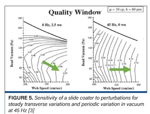
Deviations in coatweight may be caused by mechanical defects in the coater (e.g., taper and deflections of rolls); however, they also exhibit periodicity in either the machine direction (MD) or the transverse direction (TD). Deviations can be measured directly using a high-resolution (e.g., capacitance) gauge or the sensitivity (amplitude ratio) to disturbances can be predicted numerically [5]. MD gauging gives a direct readout of the effect of all existing variations, and the frequency of mechanical systems can be calculated to pinpoint the sources of variation. Numerical methods can separate out the effects of specific variations. Figure 5 shows the computed sensitivity of a slide coater to MD disturbances caused by vacuum fluctuations (45 Hz). For TD variations, the wavelength (or wavenumber) is determined by fluid mechanics, and numerical methods can predict the most dangerous mode as well as help you fi ne-tune the formulation and process.
Figure 3 also shows the sensitivity of a slide coater to TD disturbances at the most dangerous wavenumber (2.5). For this formulation, at low speed, transverse variations are minimized by running near the middle of the vacuum range, while at high speed, it is better to run in the lower part of the window – between 70 and 80 Pa (0.28 to 0.32 “WC [water column]) vacuum. MD
variations, on the other hand are minimized at all speeds by running around 80 Pa (and both sets of disturbances are maximized by running at higher speed). The specifics apply only to this formulation. What is important is the computed tolerance for the sweet spot (+ 0.02 “WC): This is the kind of precision you will eventually need for optimization and vacuum control.
Measurement of coatweight variations inside the coating window is done with a high-resolution coatweight gauge. Contour plots analogous to Figure 5 are constructed by running designed experiments (using “response surface methodologies”). The reason that the methodology for stage one is different from stage two is that the statistical methods assume you can measure each point on the design and get a unique response from that. Attempting to run outside the window and the possibility that the response may depend on how you got to that point (hysteresis) are problematic for statistical analysis: Use your stage one mapping to ensure the statistical investigation is conducted over an operable range and not confounded by hysteresis.
Managing the coating window
Mapping the coating window can help you find the sweet spot of the base case; however, the larger payoff usually requires making subtle adjustments to the formulation (% solids, surfactant level and solvent blend) and process settings (gap, off set, angle, etc.). But there can be many variables that affect maximum coating speed, quality and processing latitude.
Once the base case is mapped, map the interplay of other variables to optimize coating latitude and quality. For example, many optical coaters choose to run slot-die coaters without a vacuum box to avoid the effects shown for a slide coater in Figure 5. In this case, the approximations that led to Figure 3 also can be used to find the maximum speed that can be coated without a vacuum box as a function of dynamic contact angle. Statistical fits to the theory can be used to optimize productivity. The details of window management depend on the detailed design of the coater and the application.
This final stage of coating-window management must be directed by engineering judgment, not a scripted procedure. The optimization stage can be time-consuming and expensive; however, this is where the major improvements in quality and productivity typically occur.
Conclusion
Most industrial operations operate near a constraint or at an intersection of constraints determined by multiple formulation and process parameters. Knowing how to optimize productivity and quality while manipulating those constraints is critical to developing a competitive advantage. Having maps to guide you is invaluable.
References
1. Coyle, D.J., “Knife and Roll Coating” in Liquid Film Coating: Scientifi c principles and their technological implications. London” Kistler, S. F. (Editor) and Schweizer, P. N. (Editor), London” Chapman and Hall (1997)
2. Lightfoot, E.J., “Troubleshooting and defect reduction in coated products,” Converting Quarterly 2020 Q1, pp. 52-54
3. Ding, X., Liu, J. and Harris, T.A.L. (2016), A review of the operating limits in slot-die coating processes. AIChE J., 62: 2508-2524. https://doi.org/10.1002/aic.15268
4. Hens, J. and Van Abbenyen, W., “Slide Coating” in Liquid Film Coating: Scientific principles and their technological implications. London, Kistler, S.F. (Editor) and Schweizer, P.-N. (Editor), London, Chapman and Hall (1997)
5. Christodolou, K.N., Kistler, S.F. and Schunk, P.R., “Advances in computational methods for free surface flows” in Liquid Film Coating: Scientific principles and their technological implications. London, Kistler, S.F. (Editor) and Schweizer, P.N. (Editor), London, Chapman and Hall (1997)
6. Hackler, M.A., Christodoulou, K.N., Hirschburg, R.I., Lightfoot, E J., “Frequency response of coating flows to small three-dimensional disturbances by super-computeraided analysis,” Paper 43d, AIChE Spring National Meeting, New Orleans, 1992
E.J. (Ted) Lightfoot, principal at Ted Lightfoot LLC, holds a B.S.E. from Princeton and an M.S. and Ph.D. from the University of Illinois at Urbana Champaign (all in Chemical Engineering). He worked for DuPont for over 35 years in the photographic business, casting, coating and laminating fluoropolymer films, and making optical films (as well as some emerging technologies). Ted’s experience includes R&D, plant support, being a Six Sigma Black Belt for Growth and helping customers develop and troubleshoot processes and products comprising DuPont materials. He is currently a consultant, writer, speaker and teaches short courses. Ted can be reached at 716-449-4455, email: TedLightfoot.LC@ gmail.com or www.TedLightfoot.com.
Original article can be found online here.